Extracting Satellite Arcs

This page describes the extract_arcs module and highlights some useful features. It was produced for version 3.19.2 and may be out of date.

Please visit the function definition page to view the most recent API reference.

Overview 

The extract_arcs module provides a clean API for accessing SNR/geometry data and associated metadata of individual satellite arcs within an SNR file.

Two convenience functions cover the most common workflows:

Function	Use when you have…
`extract_arcs_from_station()`	a station name, year and day-of-year
`extract_arcs_from_file()`	a direct path to an SNR file

Quick Start 

import numpy as np
from gnssrefl.extract_arcs import extract_arcs_from_station

# Extract arcs across all available frequencies
arcs = extract_arcs_from_station('mchl', 2025, 11)

print(f'{len(arcs)} arcs found')
for meta, data in arcs[:3]:
    print(f"  sat {meta['sat']:3d}  freq {meta['freq']:3d}  "
          f"{meta['arc_type']:7s}  az={meta['az_min_ele']:5.1f}  "
          f"delT={meta['delT']:.1f} min  pts={meta['num_pts']}")
# 457 arcs found
#   sat 202  freq 206  rising   az=290.4  delT=128.0 min  pts=257
#   sat 203  freq 206  rising   az=219.8  delT=67.0 min  pts=135
#   sat 203  freq 206  setting  az=330.0  delT=84.0 min  pts=169

You can also request specific frequencies, or pass a path directly:

arcs = extract_arcs_from_station('mchl', 2025, 11, freq=1)        # L1 only
arcs = extract_arcs_from_station('mchl', 2025, 11, freq=[1, 2, 5]) # L1+L2+L5

from gnssrefl.extract_arcs import extract_arcs_from_file
arcs = extract_arcs_from_file('/path/to/ssss0110.25.snr66')        # all frequencies

Input Reference 

Some commonly used parameters. All keyword arguments below can be passed to extract_arcs_from_station(), extract_arcs_from_file(), or extract_arcs().

Parameter	Default	Description
`freq`	None (all)	GNSS frequency code: int, list of int, or None for auto-detect
`e1` / `e2`	5.0 / 25.0	Elevation angle mask (deg)
`ellist`	None	Multiple elevation ranges (overrides e1/e2)
`azlist`	[0, 360]	Azimuth regions as pairs
`sat_list`	None (all)	Restrict to specific satellite PRNs
`min_pts`	20	Minimum points per arc
`ediff`	2.0	Elevation span tolerance for QC (deg)
`polyV`	4	Polynomial order for DC removal
`pele`	[e1, e2]	Elevation range for polynomial DC removal (deg)
`buffer_hours`	0	Hours of adjacent-day data to load for midnight arcs
`filter_to_day`	True	Only keep arcs with midpoint in 0-24 h
`attach_results`	False	Match arcs to gnssir/phase output files
`screenstats`	False	Print debug information

Output Reference 

extract_arcs returns a list of (metadata, data) tuples, one per arc.

Metadata keys

Key	Type	Description
`sat`	int	Satellite PRN number
`freq`	int	Frequency code (1, 2, 5, 20, 101, 102, 201, 205, …)
`arc_num`	int	Arc index within this satellite (1, 2, …)
`arc_type`	str	`'rising'` or `'setting'`
`ele_start`	float	Minimum observed elevation angle (deg)
`ele_end`	float	Maximum observed elevation angle (deg)
`az_min_ele`	float	Azimuth at minimum elevation angle (deg)
`az_avg`	float	Mean azimuth over the arc (deg)
`time_start`	float	Start time (seconds of day)
`time_end`	float	End time (seconds of day)
`arc_timestamp`	float	Mean time of arc (hours UTC)
`num_pts`	int	Number of data points
`delT`	float	Arc duration (minutes)
`edot_factor`	float	tan(e)/edot for RHdot correction (hours/rad)
`cf`	float	Scale factor = wavelength / 2 (meters)
`gnssir_processing_results`	dict or None	gnssir result for this arc (requires `attach_results=True`)
`phase_processing_results`	dict or None	phase result for this arc (requires `attach_results=True`)
`vwc_track_results`	dict or None	VWC track data for this arc (requires `attach_results=True` and track files from `vwc -vegetation_model 2 -save_tracks T`)

Data keys

Key	Type	Description
`ele`	np.ndarray	Elevation angles (deg)
`azi`	np.ndarray	Azimuth angles (deg)
`snr`	np.ndarray	Detrended SNR (linear units, DC removed)
`seconds`	np.ndarray	Seconds of day
`edot`	np.ndarray	Elevation rate of change

Plotting Arc Data 

Using the arcs from the Quick Start, select L2C arcs for plotting:

import matplotlib.pyplot as plt

arcs = [(m, d) for m, d in arcs if m['freq'] == 20]
print(f'{len(arcs)} L2C arcs')
# 70 L2C arcs

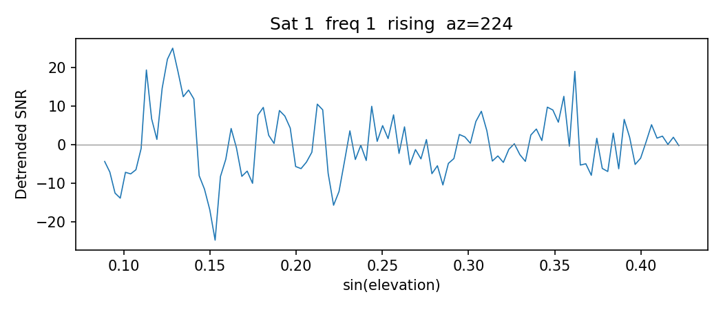
Plot 1: Detrended SNR vs sin(elevation)

This is the fundamental GNSS-IR observable. The interference pattern between the direct and reflected signals oscillates at a frequency proportional to the reflector height.

# sat 14 has one of the strongest interference patterns on this day
meta, data = [(m, d) for m, d in arcs if m['sat'] == 14][0]
x = np.sin(np.radians(data['ele']))

fig, ax = plt.subplots()
ax.plot(x, data['snr'])
ax.set_xlabel('sin(elevation)')
ax.set_ylabel('Detrended SNR')
ax.set_title(f"Sat {meta['sat']}  freq {meta['freq']}  "
             f"{meta['arc_type']}  az={meta['az_min_ele']:.0f}")
fig.tight_layout()
plt.show()

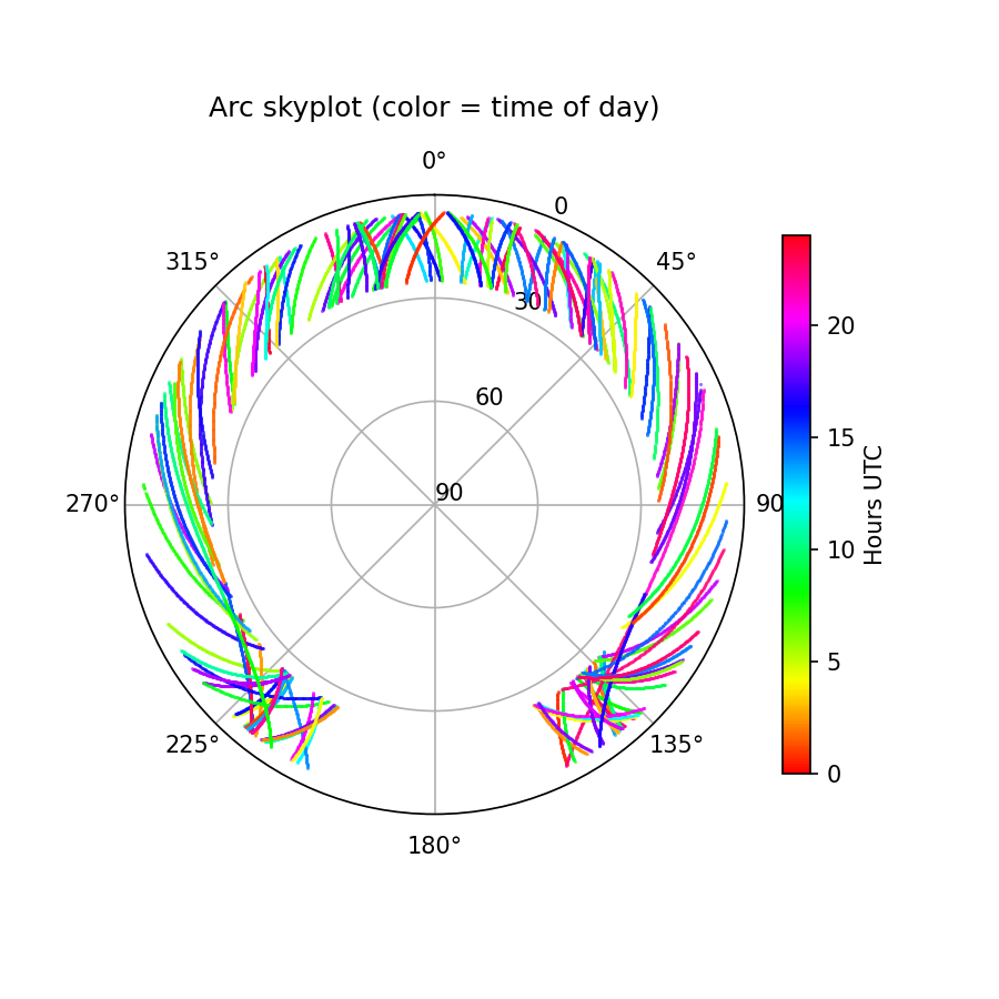
Plot 2: Polar skyplot 

Shows spatial coverage and which azimuths are observed at each time of day.

fig, ax = plt.subplots(subplot_kw={'projection': 'polar'}, figsize=(6, 6))
ax.set_theta_zero_location('N')
ax.set_theta_direction(-1)
norm = plt.Normalize(0, 24)

for meta, data in arcs:
    az_rad = np.radians(data['azi'])
    r = 90 - data['ele']          # radial axis = zenith angle
    color = plt.cm.hsv(norm(meta['arc_timestamp']))
    ax.plot(az_rad, r, '.', color=color, markersize=1, alpha=0.6)

ax.set_ylim(0, 90)
ax.set_yticks([0, 30, 60, 90])
ax.set_yticklabels(['90', '60', '30', '0'])
ax.set_title('Arc skyplot (color = time of day)')

sm = plt.cm.ScalarMappable(cmap='hsv', norm=norm)
sm.set_array([])
fig.colorbar(sm, ax=ax, label='Hours UTC')
plt.show()

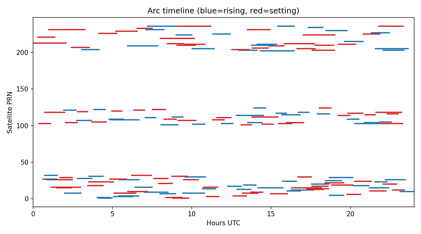
Plot 3: Arc timeline 

Shows when each satellite is observed and whether the arc is rising or setting. This motivates the midnight-crossing discussion below.

fig, ax = plt.subplots(figsize=(9, 5))
for meta, data in arcs:
    t0 = meta['time_start'] / 3600
    t1 = meta['time_end'] / 3600
    color = 'tab:blue' if meta['arc_type'] == 'rising' else 'tab:red'
    ax.plot([t0, t1], [meta['sat'], meta['sat']],
            color=color, linewidth=2, solid_capstyle='round')

ax.set_xlabel('Hours UTC')
ax.set_ylabel('Satellite PRN')
ax.set_xlim(0, 24)
ax.set_title('Arc timeline (blue=rising, red=setting)')
fig.tight_layout()
fig.show()

Linking Arcs to Processing Results 

Pass attach_results=True to match each arc back to its gnssir and phase output. Each arc’s metadata gains two new keys: gnssir_processing_results and phase_processing_results. Arcs that were rejected by QC get None.

gnssir_processing_results keys:

Key	Type	Description
`RH`	float	Reflector height (m)
`Amp`	float	LSP amplitude (volts/volts)
`PkNoise`	float	Peak-to-noise ratio
`MJD`	float	Modified Julian Date
`UTCtime`	float	UTC time (hours)
`Azim`	float	Azimuth (deg)
`eminO`	float	Observed minimum elevation (deg)
`emaxO`	float	Observed maximum elevation (deg)
`NumbOf`	int	Number of observations used
`DelT`	float	Arc duration (minutes)
`EdotF`	float	Elevation rate factor
`refr`	int	Refraction model applied (1=yes, 0=no)
`rise`	int	1 = rising, -1 = setting

phase_processing_results keys:

Key	Type	Description
`Phase`	float	Estimated phase (deg)
`Nv`	int	Number of observations used
`Azimuth`	float	Azimuth (deg)
`Ampl`	float	LSP amplitude (volts/volts)
`emin`	float	Minimum elevation (deg)
`emax`	float	Maximum elevation (deg)
`DelT`	float	Arc duration (minutes)
`aprioriRH`	float	A priori reflector height (m)
`estRH`	float	Estimated reflector height (m)
`pk2noise`	float	Peak-to-noise ratio
`LSPAmp`	float	LSP amplitude at estimated RH

Plot 4: Highest vs lowest amplitude arc 

With the processing results attached, you can sort arcs by any QC metric and immediately plot the underlying SNR data to see why an arc scored high or low.

arcs = extract_arcs_from_station('p038', 2025, 99, attach_results=True)

matched = [(m, d) for m, d in arcs if m['gnssir_processing_results'] is not None]
print(f'{len(arcs)} arcs extracted, {len(matched)} passed QC')
# 237 arcs extracted, 50 passed GNSSIR QC

matched.sort(key=lambda x: x[0]['gnssir_processing_results']['Amp'])
hi_meta, hi_data = matched[-1]
lo_meta, lo_data = matched[0]

fig, (ax1, ax2) = plt.subplots(2, 1, figsize=(7, 5), sharex=True, sharey=True)
ax1.plot(np.sin(np.radians(hi_data['ele'])), hi_data['snr'], lw=0.8)
ax1.set_title(f"Highest: sat {hi_meta['sat']} {hi_meta['arc_type']} Amp={hi_meta['gnssir_processing_results']['Amp']:.1f} PkNoise={hi_meta['gnssir_processing_results']['PkNoise']:.1f}")
ax2.plot(np.sin(np.radians(lo_data['ele'])), lo_data['snr'], lw=0.8, color='tab:orange')
ax2.set_title(f"Lowest: sat {lo_meta['sat']} {lo_meta['arc_type']} Amp={lo_meta['gnssir_processing_results']['Amp']:.1f} PkNoise={lo_meta['gnssir_processing_results']['PkNoise']:.1f}")
ax2.set_xlabel('sin(elevation)')
fig.tight_layout()
plt.show()

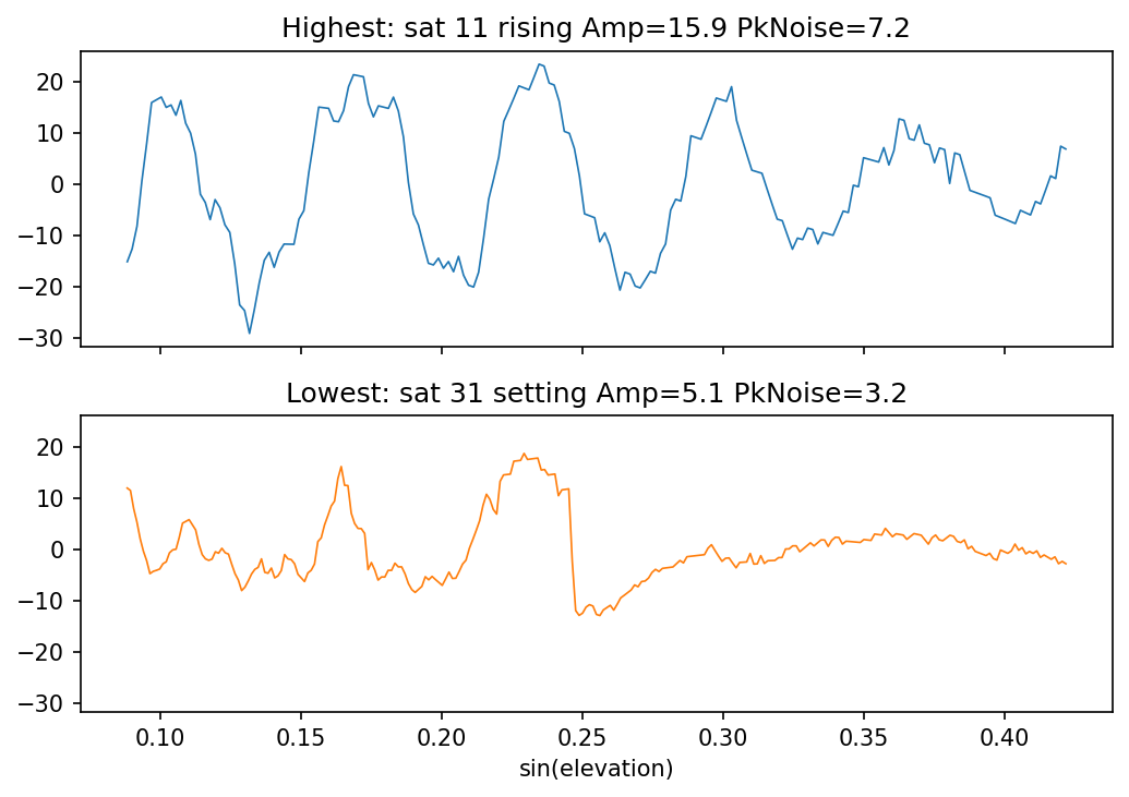
The lowest amplitude arc (Amp=5.1, PkNoise=3.2) is borderline. The interference pattern is barely visible at higher elevations. Tightening the ampl or pk2noise thresholds in the JSON would reject arcs like this.

Plot 5: Comparing arcs across days 

Extracting the same satellite track on consecutive days lets you visualize day-to-day changes in the interference pattern. Here we pull sat 3 (setting, az~187) on p038 DOY 183 and 184, 2023:

p038_doy183 = extract_arcs_from_station('p038', 2023, 183, freq=20, sat_list=[3], attach_results=True)
p038_doy184 = extract_arcs_from_station('p038', 2023, 184, freq=20, sat_list=[3], attach_results=True)

fig, ax = plt.subplots(figsize=(7, 3))
for arcs, doy in [(p038_doy183, 183), (p038_doy184, 184)]:
    # sat 3 arc nearest az=187
    meta, data = min(arcs, key=lambda a: abs(a[0]['az_min_ele'] - 187))
    p = meta['phase_processing_results']
    ax.plot(np.sin(np.radians(data['ele'])), data['snr'], label=f"DOY {doy}  phase={p['Phase']:.0f}" + r"$^\circ$")
ax.set_xlabel('sin(elevation)')
ax.set_ylabel('Detrended SNR')
ax.set_title(f"p038 sat 3 {meta['arc_type']} az={meta['az_min_ele']:.0f}" + r"$^\circ$" + " - consecutive days")
ax.legend()
fig.tight_layout()
plt.show()

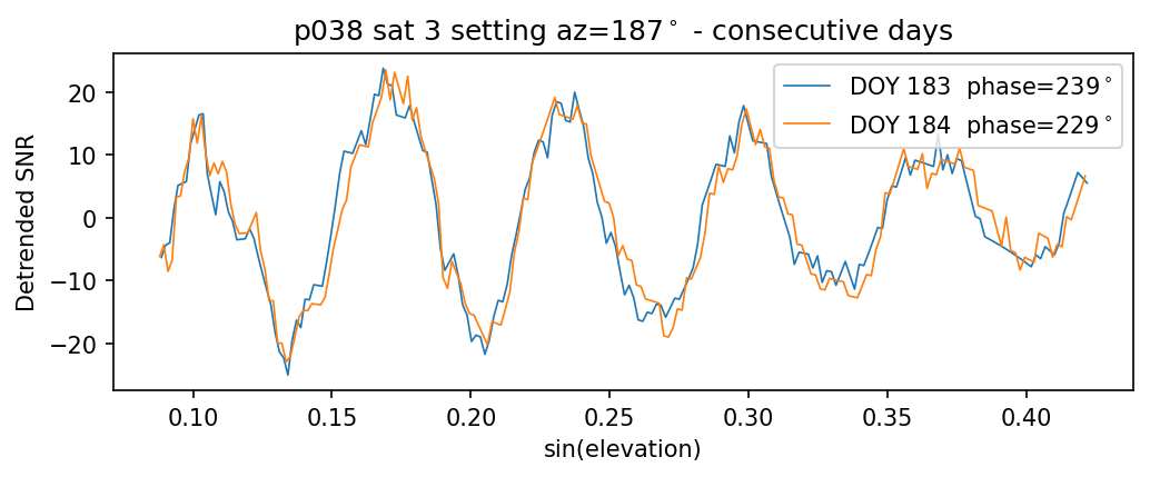
The interference patterns are nearly identical but shifted. The 10 degree phase change between these two days may correspond to a change in near-surface soil moisture.

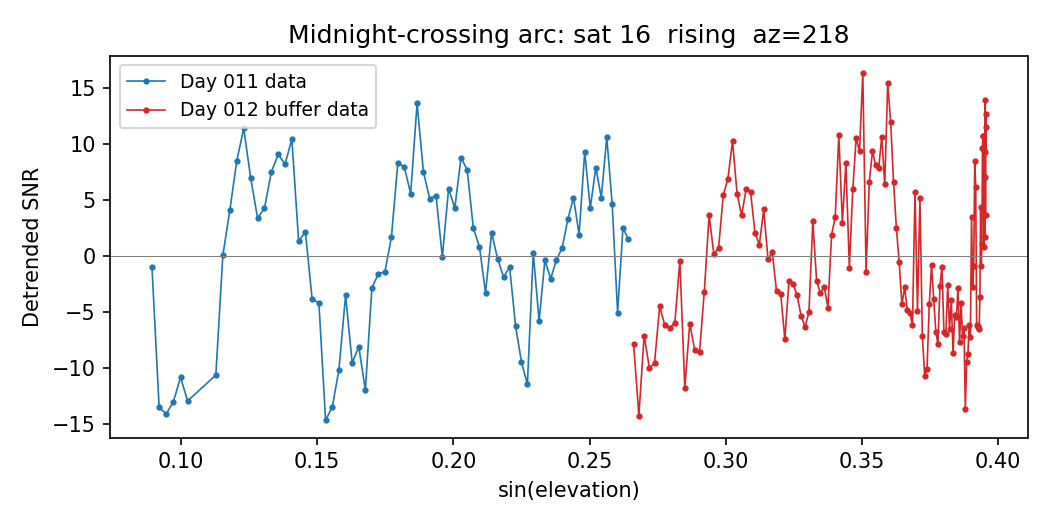
Midnight-Crossing Arcs 

SNR files cover one UTC day. Arcs in progress at midnight get split across two files and are usually too short to pass QC. Pass buffer_hours=2 to automatically load adjacent-day data with shifted time tags (previous day gets negative seconds, next day exceeds 86400). Adjacent-day files are located by name from the standard $REFL_CODE/{yyyy}/snr/{station}/ directory; a warning is printed if either neighbour is missing.

# Buffer by two hours before/after the specified day
arcs = extract_arcs_from_station('mchl', 2025, 10, freq=20, buffer_hours=2)

# Find a midnight-crossing arc and plot it
for meta, data in arcs:
    secs = data['seconds']
    if np.any(secs > 86400):  # has next-day buffer data
        main = secs <= 86400
        buf = ~main
        x = np.sin(np.radians(data['ele']))
        plt.plot(x[main], data['snr'][main], 'o-', ms=2, lw=0.8, label='Day N')
        plt.plot(x[buf], data['snr'][buf], 'o-', ms=2, lw=0.8, label='Day N+1 buffer')
        plt.legend(); plt.xlabel('sin(elevation)'); plt.ylabel('Detrended SNR')
        break

When processing consecutive days with buffer_hours, filter_to_day=True (the default) prevents double-counting by only returning arcs whose midpoint falls within 0-24 hours UTC.

Working with Raw Arrays 

If you already have SNR data as a numpy array (e.g. from custom loading or testing), you can call extract_arcs() directly:

arcs = extract_arcs(snr_array)                       # all frequencies
arcs = extract_arcs(snr_array, freq=1, e1=5, e2=25)  # L1 only

The array must have columns: [sat, ele, azi, seconds, edot, snr_col1, ...]. This is the same format returned by read_snr() and np.loadtxt() on an SNR file.