Understanding

Overview

gnssrefl is an open source/python version of my GNSS interferometric reflectometry (GNSS-IR) code.

If you would like to try out reflectometry without installing the code

I recommend you use this web app. It can show you representative results with minimal constraints. It should provide results in less than 10 seconds.

Goals

The goal of the gnssrefl python repository is to help you compute (and evaluate) GNSS-based reflectometry parameters using geodetic data. This method is often called GNSS-IR, or GNSS Interferometric Reflectometry. There are three main modules:

rinex2snr translates RINEX files into SNR files needed for analysis.
gnssir computes reflector heights (RH) from SNR files.
quickLook gives you a quick (visual) assessment of a file without dealing with the details associated with gnssir. It is not meant to be used for routine analysis. It also helps you pick an appropriate azimtuh mask and quality control settings.

There are also various utilities you might find to be useful. If you are unsure about why various restrictions are being applied, it is really useful to read Roesler and Larson (2018) or similar. You can also watch some background videos on GNSS-IR at youtube.

Philosophy

In geodesy, you don’t really need to know much about what you are doing to calculate a reasonably precise position from GPS data. That’s just the way it is. (Note: that is also thanks to the hard work of the geodesists that wrote the computer codes). For GPS/GNSS reflections, you need to know a little bit more - like what are you trying to do? Are you trying to measure water levels? Then you need to know where the water is! (with respect to your antenna, i.e. which azimuths are good and which are bad). Another application of this code is to measure snow accumulation. If you have a bunch of obstructions near your antenna, you are responsible for knowing not to use that region. If your antenna is 10 meters above the reflection area, and the software default only computes answers up to 6 meters, the code will not tell you anything useful. It is up to you to know what is best for the site and modify the inputs accordingly. I encourage you to get to know your site. If it belongs to you, look at photographs. If you can’t find photographs, use Google Earth. You can also try using my google maps web app interface.

Signals and Sources

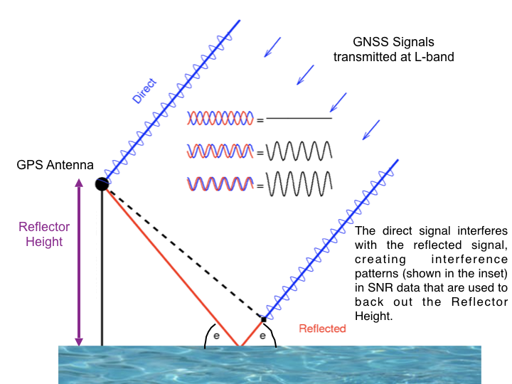
To summarize, direct (blue) and reflected (red) GNSS signals interfere and create an interference pattern that can be observed in GNSS Signal to Noise Ratio (SNR) data as a satellite rises or sets. The frequency of this interference pattern is directly related to the height of the GNSS antenna phase center above the reflecting surface, or reflector height RH (purple). The primary goal of this software is to measure RH. This parameter is directly related to changes in snow height and water levels below a GNSS antenna. This is why GNSS-IR can be used as a snow sensor and tide gauge. GNSS-IR can also be used to measure soil moisture, but the code to estimate soil moisture is not as strongly related to RH as snow and water. We will be posting the code you need to measure soil moisture later in the year.

This code is meant to be used with Signal to Noise Ratio (SNR) data. This is a SNR sample for a site in the the northern hemisphere (Colorado) and a single GPS satellite. The SNR data are plotted with respect to time - however, we have also highlighted in red the data where elevation angles are less than 25 degrees. These are the data used in GNSS Interferometric Reflectometry GNSS-IR. You can also see that there is an overall smooth polynomial signature in the SNR data. This represents the dual effects of the satellite power transmission level and the antenna gain pattern. We aren’t interested in that so we will be removing it with a low order polynomial (and we will convert to linear units on y-axis).

After that polynomial is removed, we will concentrate on the rising and setting satellite arcs. That is the red parts on the left and right.

Below you can see those next two steps. On the top is the “straightened” SNR data. Instead of time, it is plotted with respect to sine of the elevation angle. It was shown a long time ago by Penina Axelrad that the frequency extracted from these data is representative of the reflector height. Here a periodogram was used to extract this frequency, and that is shown below, with the x-axis units changed to reflector height. In a nutshell, that is what this code does. It figures out the rising and setting satellite arcs in all the azimuth regions you have said are acceptable. It does a simple analysis (removes the polynomial, changes units) and uses a periodogram to look at the frequency content of the data. You only want to report RH when you think the peak on the periodogram is significant. There are many ways to do this - we only use two quality control metrics:

is the peak larger than a user-defined value (amplitude of the dominant peak in your periodogram)
is the peak divided by a “noise” metric larger than a user-defined value. The code calls this the peak2noise.

The Colorado SNR example is for a fairly planar field where the RH for the rising and setting arc should be very close to the same name. What does the SNR data look like for a more extreme case? Shown below is the SNR data for Peterson Bay, where the rising arc (at low tide) has a very different frequency than during the setting arc (high tide). This gives you an idea of how the code can be used to measure tides.

Considerations

A couple common sense issues: one is that since you define the noise region, if you make it really large, that will artificially make the peak2noise ratio larger. I have generally used a region of 6-8 meters for this calculation. So in the figure above the region was for 0-6 meters. The amplitude can be tricky because some receivers report low SNR values, which then leads to lower amplitudes. The default amplitude values are for the most commonly used signals in GNSS-IR (L1, L2C, L5, Glonass, Galileo, Beidou). The L2P data used by geodesists are generally not useable for reasons to be discussed later.

Even though we analyze the data as a function of sine of elevation angle, each satellite arc is associated with a specific time period. The code keeps track of that and reports it in the final answers. It also keeps track of the average azimuth for each rising and setting satellite arc that passes quality control tests.

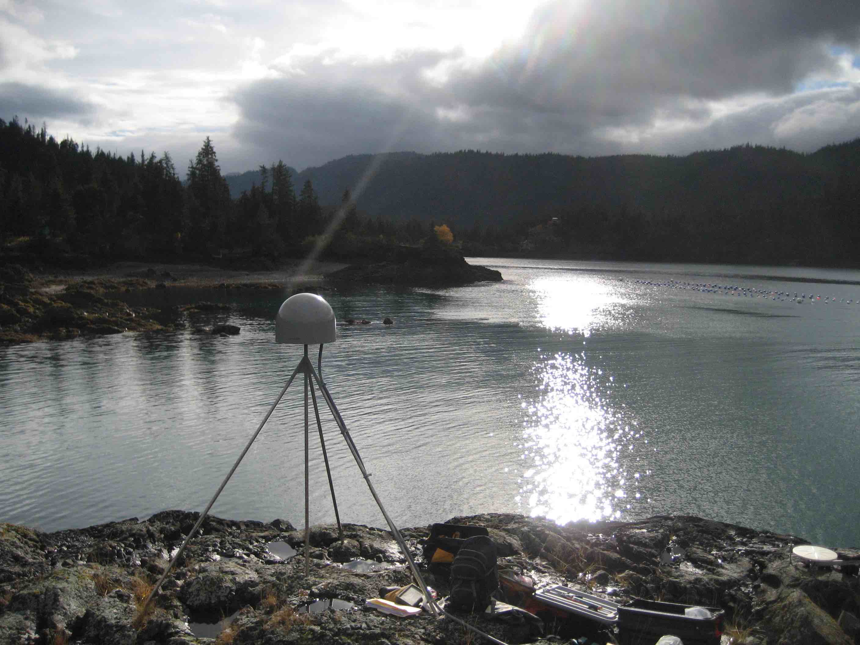
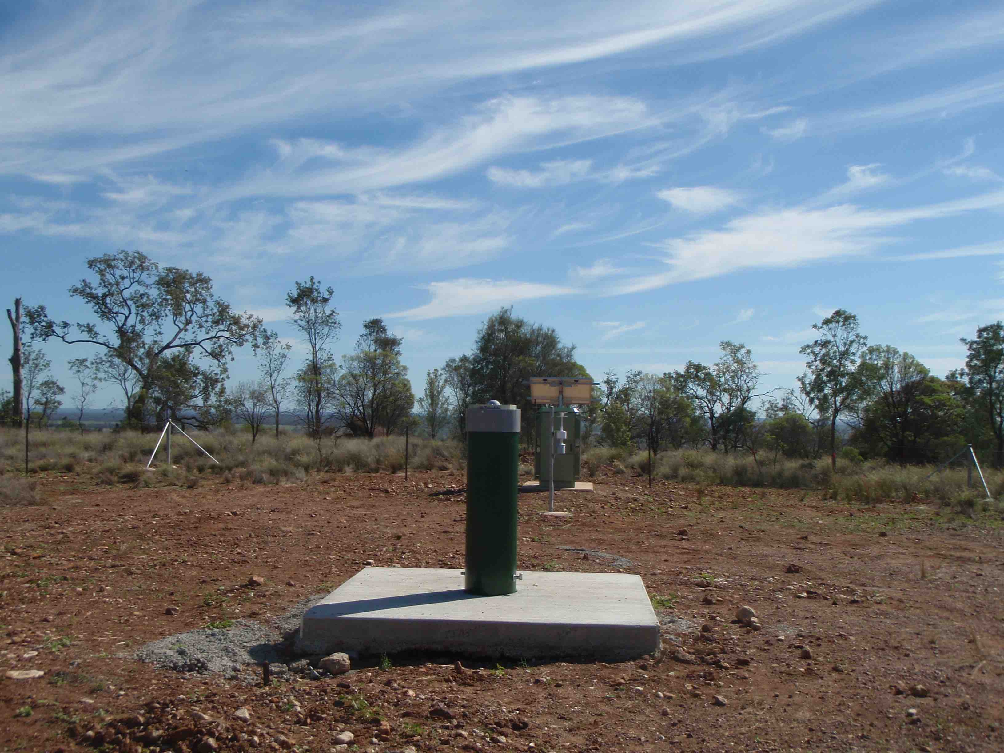
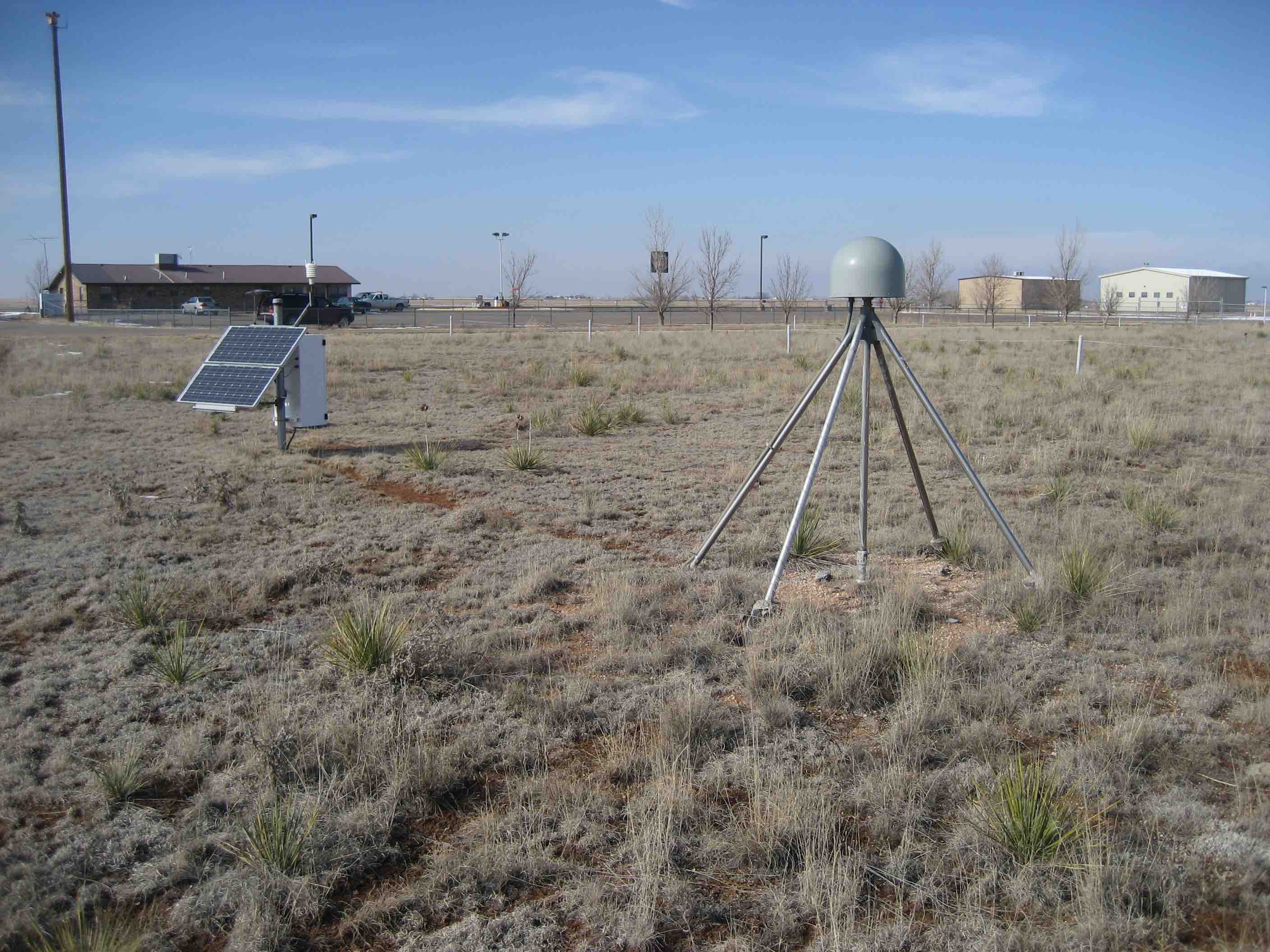
What do these satellite reflection zones look like? Below are photographs and reflection zone maps for two standard GNSS-IR sites, one in the northern hemisphere and one in the southern hemisphere.

Mitchell, Queensland, Australia	Portales, New Mexico, USA

Each one of the yellow/blue/red/green/cyan clusters represents the reflection zone for a single rising or setting GPS satellite arc. The colors represent different elevation angles - so yellow is lowest (5 degrees), blue (10 degrees) and so on. The missing satellite signals in the north (for Portales New Mexico) and south (for Mitchell, Australia) are the result of the GPS satellite inclination angle and the station latitudes. The length of the ellipses depends on the height of the antenna above the surface - so a height of 2 meters gives an ellipse that is smaller than one that is 10 meters. In this case we used 2 meters for both sites - and these are pretty simple GNSS-IR sites. The surfaces below the GPS antennas are fairly smooth soil and that will generate coherent reflections. In general, you can use all azimuths at these sites.

Now let's look at a more complex case, station ross on Lake Superior. Here the goal is to measure water level. The map image (panel A) makes it clear that unlike Mitchell and Portales, we cannot use all azimuths to measure the lake. To understand our reflection zones, we need to know the approximate lake level. That is a bit tricky to know, but the photograph (panel B) suggests it is more than the 2 meters we used at Portales - but not too tall. We will try 4 meters and then check later to make sure that was a good assumption.

A. Map view of station ROSS	B. 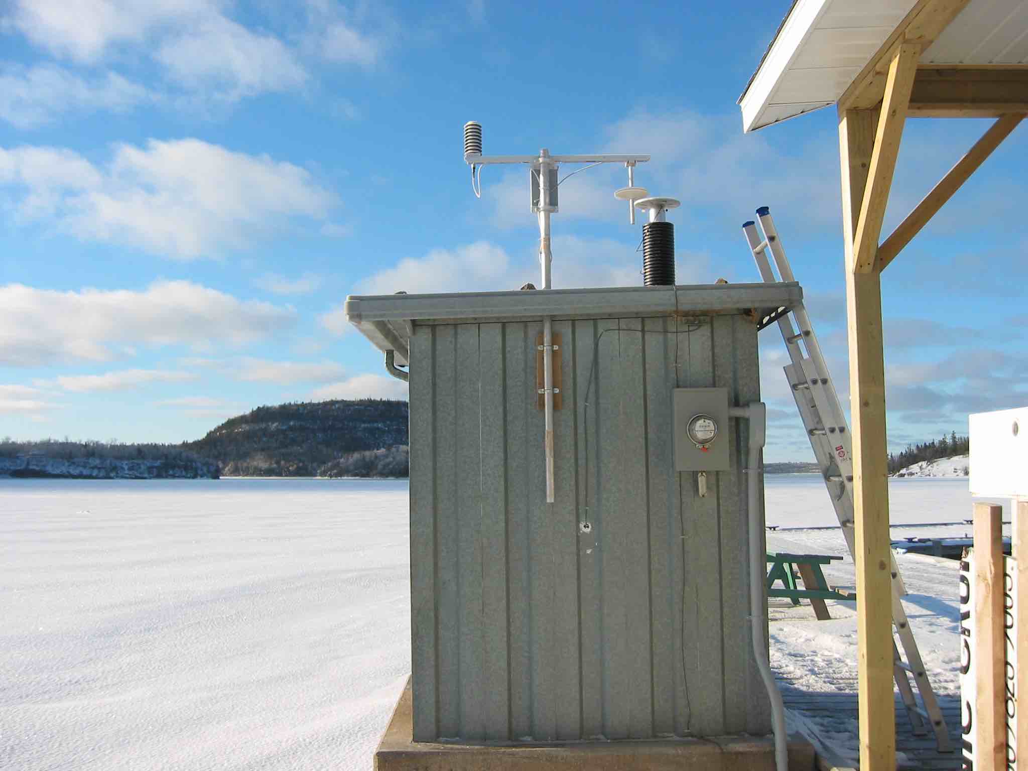Photograph of station ROSS
C. Reflection zones for GPS satellites at elevation angles of 5-25 degrees for a reflector height of 4 meters.	D. Reflection zones for GPS satellites at elevation angles of 5-15 degrees for a reflector height of 4 meters.

Again using the reflection zone web app, we can plot up the appropriate reflection zones for various options. Since ross has been around a long time, http://gnss-reflections.org has its coordinates in a database. You can just plug in ross for the station name and leave latitude/longitude/height blank. You do need to plug in a RH of 4 since mean sea level would not be an appropriate reflector height value for this case. Start out with an azimuth range of 90 to 180 degrees. Using 5-25 degree elevation angles (panel C) looks like it won’t quite work - and going all the way to 180 degrees in azimuth also looks it will be problematic. Panel D shows a smaller elevation angle range (5-15) and cuts off azimuths at 160. These choices appear to be better than those from Panel C.
It is also worth noting that the GPS antenna has been attached to a pier - and boats dock at piers. You might very well see outliers at this site when a boat is docked at the pier.

Note: we now have a refl_zones tool in the gnssrefl package.

Once you have the code set up, it is important that you check the quality of data. This will also allow you to check on your assumptions, such as the appropriate azimuth and elevation angle mask and reflector height range. This is one of the reasons quickLook was developed.