Homework 2 Solution
(Solutions and figures were generated using gnssrefl v1.5.3)
Make SNR file for gls1, 2012, doy 100 quickLook*
rinex2snr gls1 2012 100 -archive unavco
Run quickLook
quickLook gls1 2012 100
This makes two plots.
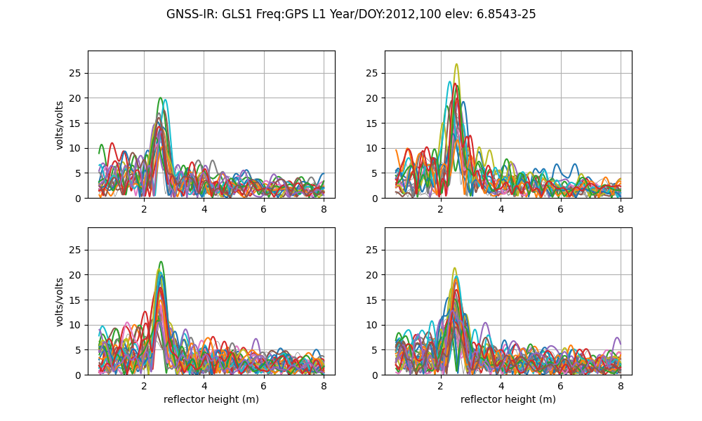

Looking at the QC metrics plots created by quickLook, do you have some ideas on how to change the azimuth mask angles?
Now make SNR files for gls1 for the all of 2012.
rinex2snr gls1 2012 1 -archive unavco -doy_end 366 -weekly True
We will next analyze a year of L1 GPS reflection data from gls1. We will use the default minimum and maximum reflector height values (0.5 and 8 meters). But for the reasons previously stated, you will want to set a minimum elevation angle of 7 degrees. We also specify that we only want to use the L1 data. We will get the coordinates from UNR and specify the azimuth mask
gnssir_input gls1 -l1 True -e1 7 -peak2noise 3 -ampl 8 -azlist2 40 330
Now that you have SNR files and json inputs, you can go ahead and
estimate reflector heights for the year 2012 using gnssir.
Note that it is normal to see ‘Could not read the first SNR file:’ because we
only created SNR files once a week.
gnssir gls1 2012 1 -doy_end 366
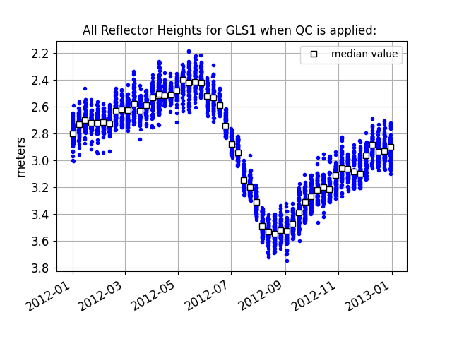
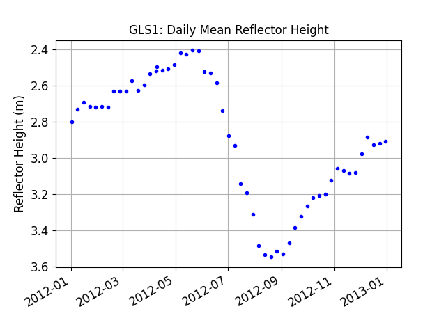
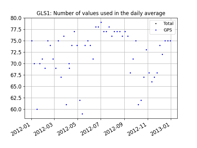
Now you can use the daily_avg tool to compute a daily average reflector height for gls1.
Try setting the median filter to 0.25 meters and individual tracks to 30.
daily_avg gls1 0.25 30
This code produces three plots and a daily average (txt or csv) file.
This is all the individual RH:
This is the daily average after outliers have been removed:
This lets you know how many arcs went into each day’s average:
Note that RH is plotted on the y-axis with RH decreasing rather than increasing. Why do you think we did that?
Most people are interested in snow accumulation, so reversing the y-axis accommodates that.