Stillwater, Oklahoma
metadata
Station Name: okl2
Location: Oklahoma, USA
Archive: UNAVCO
Ellipsoidal Coordinates:
Latitude: 36.063492 degrees
Longitude: -97.216964 degrees
Height: 328 meters
This use case demonstrates the advanced vegetation model (model 2) for soil moisture estimation at a well-studied site in Oklahoma with significant vegetation effects.
Background
Station okl2 was analyzed as part of the original PBO H2O network and has been used extensively for validating GNSS-IR soil moisture algorithms. The site experiences significant seasonal vegetation that requires correction to obtain accurate soil moisture estimates.
Step 1: GNSS-IR
Begin by generating the SNR files using the special archive for L2C data:
rinex2snr okl2 2012 1 -doy_end 366 -rate high -dec 15 -par 10
We must use -rate high to locate the correct file, and I optionally add -dec 15 for smaller file sizes and -par 10 for parallel downloads.
Now set up the analysis strategy:
gnssir_input okl2 -fr 20
Run gnssir to estimate reflector heights:
gnssir okl2 2012 1 -doy_end 366 -par 10
Step 2: Soil Moisture with Simple Model (Model 1)
First, let’s run the standard simple vegetation model for comparison.
Pick the satellite tracks:
vwc_input okl2 2012
Estimate phase for each satellite track:
phase okl2 2012 1 -doy_end 366 -par 10
Convert phase to volumetric water content using the simple model (default):
vwc okl2 2012
This produces the standard VWC output using model 1 (simple vegetation correction). Copy the file so it is not overwritten by the next step: $REFL_CODE/Files/okl2/okl2_vwc_L2_24hr+0.txt
Step 3: Soil Moisture with Advanced Model (Model 2)
Now run the advanced vegetation model:
vwc okl2 2012 -vegetation_model 2
The advanced model applies Clara Chew’s track-level KNN correction algorithm as described in DOI 10.1007/s10291-015-0462-4.
We can plot the results of each method to compare them:
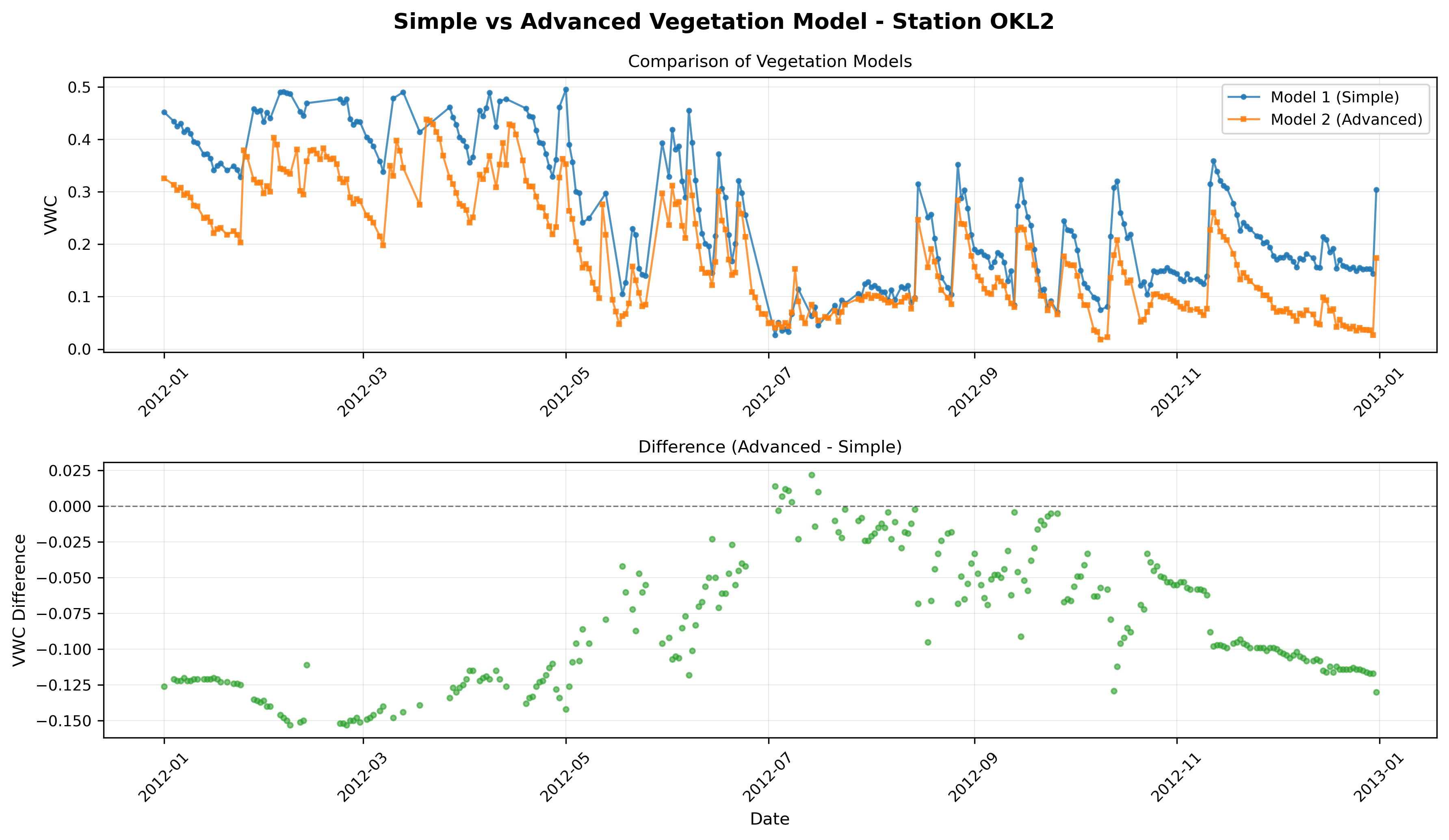
Key Ideas
Model 1 (Simple):
First aggregate measurements into daily (or subdaily) bins
Then take the average phase of every measurement in the bin
Finally, convert that averaged phase value to VWC by a fixed scalar (1.48)
Model 2 (Advanced):
This model determines track-by-track corrections at the phase level, prior to VWC conversion.
The phase -> VWC conversion scaler is also variable (this is the “slope correction”)
Both the phase and slope corrections are found from a lookup table (created by Clara Chew)
The corrections are determined based on a smoothed value of (1) amplitude of interference pattern, (2) amplitude of LSP peaks, and (3) effective RH.
Each of these inputs will change throughout the year as vegetation structure and density changes
Saving Individual Track Data
To save detailed track-level data for further analysis:
vwc okl2 2012 -vegetation_model 2 -save_tracks T
Individual track files are saved to:
$REFL_CODE/Files/okl2/individual_tracks/