Homework 3 Solution

(Solutions and figures were generated using gnssrefl v1.5.3)

Make SNR data. The only required inputs are the station name (ross), the year (2020) and day of year (150)

rinex2snr ross 2020 150

Once you have successfully created a SNR file, run quickLook.

quickLook ross 2020 150

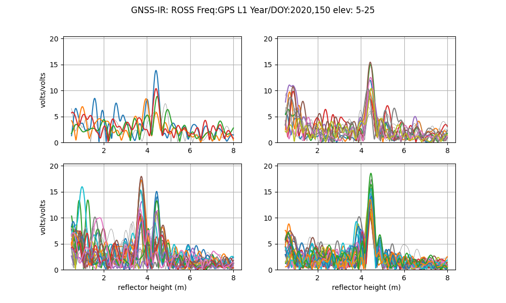
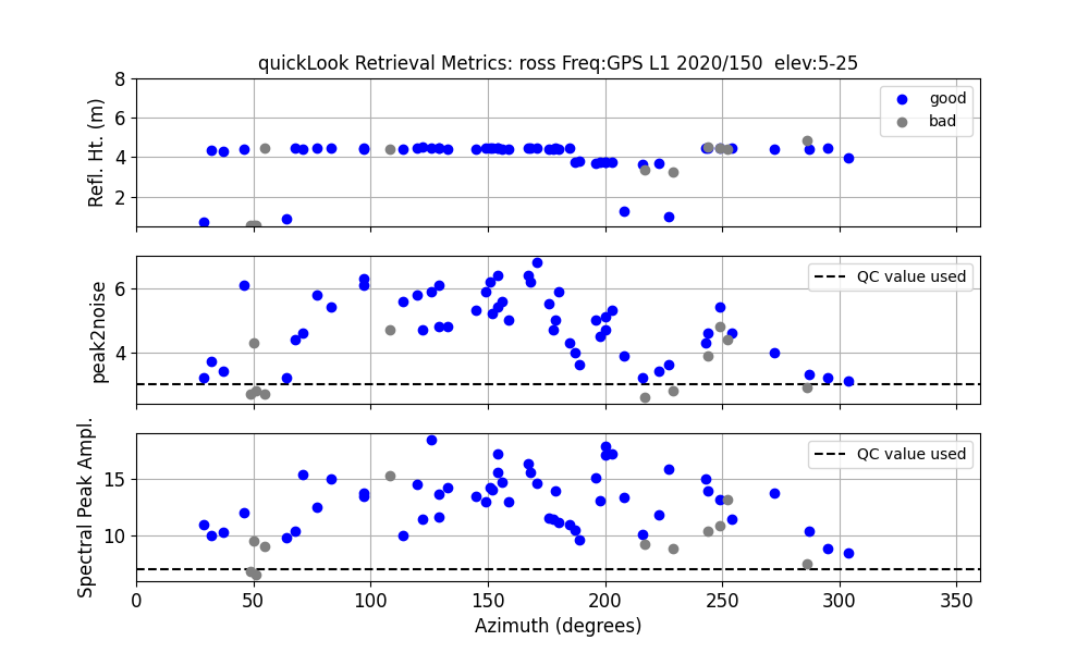
From these plots, how does the correct RH value compare with the one you assumed earlier when you were trying out the webapp? How about the azimuths? Go back to the reflection zone webapp and make sure you are happy with your azimuth and elevation angle selections.

Next we need to save our gnssir analysis strategy

I shifted the min and max RH to better accommodate the main signal from ~4.5 meters. I also limited elevation angles to 5-15 and used the peak2noise from the quickLook (which is 3). I use azimuths from the southeast region and get coordinates from UNR.

gnssir_input ross -l1 True -h1 2 -h2 8 -e1 5 -e2 15 -peak2noise 3 -azlist2 90 180

Now analyze data for the year 2020. First you need to make the snr files:

rinex2snr ross 2020 120 -doy_end 290 -weekly True

Then use the SNR data to estimate RH:

gnssir ross 2020 120 -doy_end 290

Then create a daily average RH:

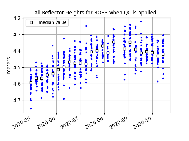
daily_avg ross 0.25 15

The daily_avg code produces multiple plots. Individual RH estimates:

The daily average for RH:

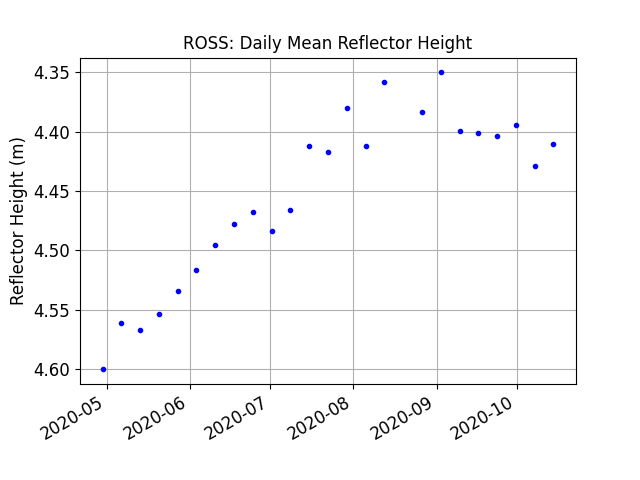
You can compare these retrievals with the NRCAN tide gauge data for Rossport. To see another Canadian lake level example, see the use case for mchn.